2011 年,柯普出版了《激情之夜:人和机器所作的俳句两千首》( Comes
the Fiery Night: 2000 Haiku by Man and
Machine),其中有一部分是安妮写的,其他则来自真正的诗人。但书中并未透露具体篇目的作者是谁。如果你认为自己一定可以看出人类创作与机器作品的差异,欢迎挑战。
It is such a general and powerful tool for combining information in
the presence of uncertainty.
What is it?
You can use a Kalman filter in any place where you have
uncertain information about some dynamic system, and
you can make an educated guess about what the system is
going to do next.
Kalman filters are ideal for systems which are continuously changing.
They have the advantage that they are light on memory (they don’t need
to keep any history other than the previous state), and they are very
fast, making them well suited for real time problems and embedded
systems.
It could be data about the amount of fluid in a tank, the temperature
of a car engine, the position of a user’s finger on a touchpad, or any
number of things you need to keep track of.
How a Kalman filter sees
your problem
The Kalman filter assumes that both variables are random and Gaussian
distributed. Each variable has a mean value 𝜇, which is the center of
the random distribution (and its most likely state), and a variance 𝜎2,
which is the uncertainty.
截屏 2021-03-23
下午 8.36.39.png
从参数之间的关联发掘更多信息:比如机器人的速度和位置,如果速度快,那么位置可能就比较远。
This kind of relationship is really important to keep track of,
because it gives us more information: One measurement tells us
something about what the others could be. And that’s the goal
of the Kalman filter, we want to squeeze as much information from our
uncertain measurements as we possibly can!
参数之间的相关性,可以用协方差矩阵 (covariance matrix)
来表示,即矩阵中的每个元素 ∑ij 表示第 i 个和第 j
个状态变量之间的相关度。注意,协方差矩阵是一个对称矩阵,这意味着可以任意交换
i 和 j。
This correlation is captured by something called a covariance
matrix.
Describing the problem
with matrices
We need some way to look at the current state (at time k-1) and
predict the next state at time k. We can represent this prediction step
with a prediction matrix, Fk.
请注意,预测矩阵要求严格反映运动的特征,要求预测准确,不能模糊。
For prediction matrix, it takes every point in our
original estimate and moves it to a new predicted location, which is
where the system would move if that original estimate was the
right one.
图片
不太理解这个公示是如何推导出来的,数学的理论知识不够踏实。
screen shot 2021-03-24 at
20.14.01.png
External influence
外部系统的影响
There might be some changes that aren’t related to the state itself —
the outside world could be affecting the system.
control matrix
control vector
External uncertainty
Everything is fine if the state evolves based on its own properties.
Everything is still fine if the state evolves based on external forces,
so long as we know what those external forces are.
如何应对外界的不确定性,比如四旋翼控制中的风影响。
We can model the uncertainty associated with the “world” (i.e. things
we aren’t keeping track of) by adding some new uncertainty after every
prediction step * Every state in our original estimate could have moved
to a range of states.
图片讲解
In other words, the new best estimate is a prediction made from
previous best estimate, plus a correction for known external
influences.
And the new uncertainty is predicted from the old uncertainty, with
some additional uncertainty from the environment.
Refining the estimate
with measurements
We might have several sensors which give us information about the
state of our system.
Each sensor tells us something indirect about the state— in other
words, the sensors operate on a state and produce a set of readings.
The units and scale of the reading might not be the same as the units
and scale of the state we’re keeping track of. You might be able to
guess where this is going: We’ll model the sensors with a matrix.
卡尔曼滤波的精妙处:
One thing that Kalman filters are great for is dealing with sensor
noise. In other words, our sensors are at least somewhat unreliable, and
every state in our original estimate might result in a range of sensor
readings.
From each reading we observe, we might guess that our system was in a
particular state. But because there is uncertainty, some states
are more likely than others to have have produced the reading
we saw.
We have two Gaussian blobs: One surrounding the mean of our
transformed prediction, and one surrounding the actual sensor reading we
got.
配图
We must try to reconcile our guess about the readings we’d see based
on the predicted state (pink) with a different guess based on our sensor
readings (green) that we actually observed.
If we have two probabilities and we want to know the chance that both
are true, we just multiply them together.
The mean of this distribution is the configuration for which
both estimates are most likely, and is therefore the
best guess of the true configuration given all the
information we have.
Combining Gaussians
Kalman Filter Information
Flow
Wrapping up
卡尔曼滤波用于线性系统,扩展卡尔曼滤波适用于非线性系统。
This will allow you to model any linear system
accurately. For nonlinear systems, we use the extended Kalman
filter, which works by simply linearizing the predictions and
measurements about their mean.
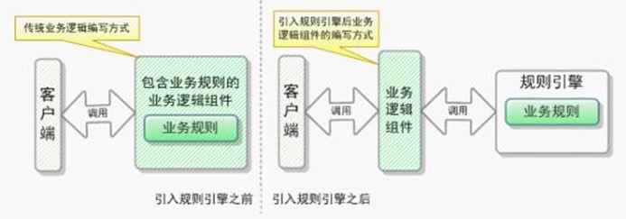
In general, the major difference between a workflow engine and a
state machine lies in focus. In a workflow engine, transition to the
next step occurs when a previous action is completed, whilst a state
machine needs an external event that will cause branching to the next
activity. In other words, state machine is event driven and workflow
engine is not.
State machine is a good solution if your system is not very complex.
You may implement it if you are capable of drawing all the possible
states as well as the events that will cause transitions to them. In
general, state machines work well for network protocols or some of the
embedded systems.
Workflow engine implementation is a good way of managing business
processes. It is the right solution for task allocation, CRM and other
complex systems. All in all, its ultimate goal is to improve business
processes and company’s efficiency. That is why it perfectly suits for
business process automation.
根据 官方网站 介绍,CLIPS
(the C Language Integrated Production System) 于 1984
年由美国航空航天局约翰逊空间中心 (NASA’s Johnson Space Center)
推出,意在克服 LISP 移植性差、开发工具和硬件成本高、嵌入性低的缺点。
Developed at NASA’s Johnson Space Center from 1985 to 1996, the C
Language Integrated Production System (CLIPS) is a rule-based
programming language useful for creating expert systems and other
programs where a heuristic solution is easier to implement and maintain
than an algorithmic solution. Written in C for portability, CLIPS can be
installed and used on a wide variety of platforms. Since 1996, CLIPS has
been available as public domain software.
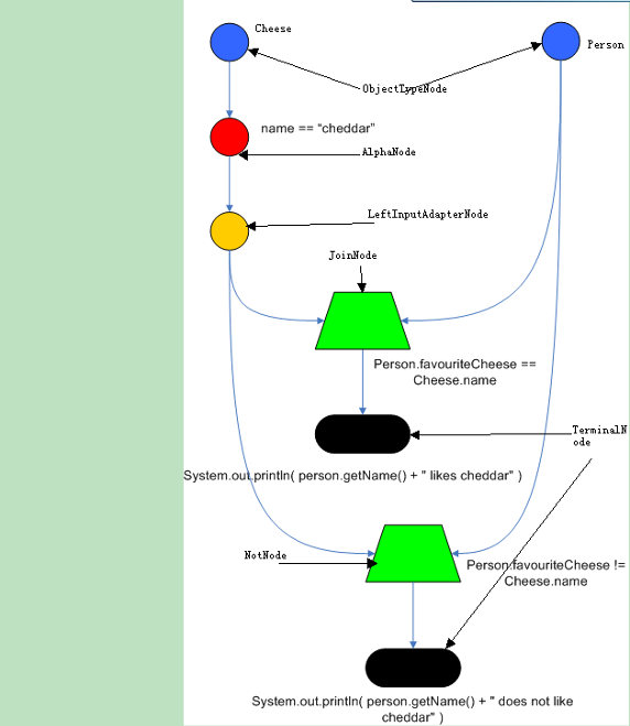
CLIPS 是一个基于 Rete 算法 的前向推理语言,用标准 C
语言编写。它具有高移植性、高扩展性、强大的知识表达能力和编程方式以及低成本等特点。
前向推理 (又叫正向推理,前向链接) 是使用推理引擎 (inference engine)
的主要方法之一,是在专家系统 (expert systems),业务和生产规则系统
(business and production rule systems) 上广泛应用的策略。
Forward chaining (or forward reasoning) is one of the two main
methods of reasoning when using an inference engine and can be described
logically as repeated application of modus ponens. Forward chaining is a
popular implementation strategy for expert systems, business and
production rule systems. The opposite of forward chaining is backward
chaining.
Forward chaining starts with the available data and uses inference
rules to extract more data (from an end user, for example) until a goal
is reached. An inference engine using forward chaining searches the
inference rules until it finds one where the antecedent (If clause) is
known to be true. When such a rule is found, the engine can conclude, or
infer, the consequent (Then clause), resulting in the addition of new
information to its data. Inference engines will iterate through this
process until a goal is reached.
The forward chainer applies rules from premises to conclusions. It
currently uses a rather brute force algorithms, select sources and rules
somewhat randomly, apply these to produce conclusions, re-insert them
are new sources and re-iterate till a stop criterion has been met.
Rete has become the basis for many popular rule engines and expert
system shells, including Tibco Business Events, Newgen OmniRules, CLIPS,
Jess, Drools, IBM Operational Decision Management, OPSJ, Blaze Advisor,
BizTalk Rules Engine, Soar, Clara and Sparkling Logic SMARTS.
The system covers multilane and single-lane autonomous driving in a
hierarchical manner: - 第一级:变道选择。The top layer
of the system is a multilane strategy that handles
lane-change scenarios by comparing lane-level
trajectories computed in parallel.
第二级:车道内的轨迹优化和速度优化。Inside the lane-level trajectory
generator, it iteratively solves path and speed optimization based on a
Frenet frame.
For path and speed optimization, a combination of dynamic
programming and spline-based quadratic programming is proposed to
construct a scalable and easy-to-tune framework to handle traffic rules,
obstacle decisions and smoothness simultaneously.
In the figure, the HD map module provides a high-definition map that
can be accessed by every on-line module. Perception and localization
modules provide the necessary dynamic environment information, which can
be further used to predict future environment status in the prediction
module. The motion planning module considers all information to generate
a safe and smooth trajectory to feed into the vehicle control
module.
1 2 3 4 5 6
graph LR
A[safety]-->B(traffic regulations)
A-->C(range coverage)
A-->D(cycle time efficiency)
A-->E(emergency safety)
C-->F(we aim to provide a trajectory with at least an eight second or two hundred meter motion planning trajectory)
In motion planner, safety is always the top priority. We consider
autonomous driving safety in, but not limited to, the following aspects:
traffic regulations, range coverage, cycle time efficiency and emergency
safety.
In addition to safety, passengers’ ride experience is also important.
The measurement of ride experience includes, but is not limited to,
scenario coverage, traffic regulation and comfort.
Typically, a multilane strategy should cover both nonpassive and
passive lane-change scenarios. * In EM planner, a nonpassive lane-change
is a request triggered by the routing module for the purpose of reaching
the final destination. * A passive lane change is defined as an ego car
maneuver when the default lane is blocked by the dynamic
environment.
We propose a parallel framework to handle both passive and nonpassive
lane changes. For candidate lanes, all obstacles and environment
information are projected on lane-based Frenet frames. Then, the traffic
regulations are bound with the given lane-level strategy. Under this
framework, each candidate lane will generate a best-possible trajectory
based on the lane-level optimizer. Finally, a cross-lane trajectory
decider will determine which lane to choose based on both the cost
functional and safety rules.
Path-Speed Iterative
Algorithm
大多数自动驾驶软件运动规划的做法是,沿着车道参考线 (reference
line,通常是从高精度地图中得到车道中心线) 把单车道问题转化为 Frenet
frames with time (SLT) 问题。其中,S 指 Frenet 坐标系下的纵向,L
指横向,T 指代时间。
Many autonomous driving motion planning algorithms are developed in
Frenet frames with time (SLT) to reduce the planning dimension with the
help of a reference line.
如何在 Frenet 中找到最优轨迹是一个 3D (S+L+T)
约束优化问题,文章中提到两种做法的路线之争。在我看来,现在工业界主流前沿的做法是第二种,第一种正在被逐渐淘汰。
Finding the optimal trajectory in a Frenet frame is essentially a 3D
constrained optimization problem. There are typically two types of
approaches: direct 3D optimization methods and the path-speed decoupled
method. * [方法一:无脑优化采样] Direct methods attempt to find the
optimal trajectory within SLT using either trajectory sampling or
lattice search. + These approaches are limited by their search
complexity, which increases as both the spatial and
temporal search resolutions increase. To qualify the
time consumption requirement, one has to compromise with increasing the
search grid size or sampling resolution. Thus, the generated trajectory
is suboptimal.
[方法二:path-speed 解耦,先求 path,再解 speed] The path-speed
decoupled approach optimizes path and speed separately.
Path optimization typically considers static obstacles. Then, the speed
profile is created based on the generated path. It is possible
that the path-speed approach is not optimal with the appearance of
dynamic obstacles. However, since the path and speed are
decoupled, this approach achieves more flexibility in both path and
speed optimization.
一个负责问题,如果一旦可以分为几个小问题,或者之前已经解决的问题,那么问题整体难度就会降低下来。
Path-speed decoupled
framework
EM planner 分别迭代优化 path 和 speed。在 path
优化中,利用上一帧的速度 (speed profile from the last cycle)
来预估和低速对象障碍物的交互,然后基于生成的 path 来优化速度。
注意,实践中要减少对上一次规划轨迹的依赖。
EM planner optimizes path and speed iteratively. The speed profile
from the last cycle is used to estimate interactions with
oncoming and low-speed dynamic
obstacles in the path optimizer. Then, the generated path is
sent to the speed optimizer to evaluate an optimal speed profile.
For high-speed dynamic dynamic obstacles, EM planner prefers a
lane-change maneuver rather than nudging for safety reasons.
Decisions and Traffic
Regulations
EM planner 先做出决策 (make
decisions),再规划轨迹。决策可以输出清晰的自车意图,把非凸问题约束为凸问题,不仅减少寻找最优轨迹的搜索空间,而且允许使用凸优化问题的优化方法。
In Apollo EM planner, we make decisions prior to providing a smooth
trajectory. The decision process is designed to make on-road intentions
clear and reduce the search space for finding the optimal
trajectory.
决策的路线之争。
Many decision-included planners attempt to generate vehicle states as
the ego car decision. These approaches can be further divided into
hand-tuning decisions and model-based decisions. *
[方法一:手写规则,扩展性差] The advantage of hand-tuning decision is
its tunability. However, scalability is its limitation. In some cases,
scenarios can go beyond the hand-tuning decision rule’s description. +
When considering dozens of obstacles, the decision behavior is difficult
to be accurately described by a finite set of ego car states.
[方法二:基于模型的决策] The model-based decision approaches
generally discretize the ego car status into finite
driving statuses and use data-driven methods to tune the model.
Targeting level-4 autonomous driving, a decision module shall include
both scalability and
feasibility.
* Scalability is the scenario expression ability (i.e., the autonomous
driving cases that can be explained). + 不要过拟合 (over-fit) 一个
issue,适用性差。 * For feasibility, we mean that the generated decision
shall include a feasible region in which the ego car can maneuver
within dynamic limitations. + Both hand-tuning and
model-based decisions do not generate a collision-free trajectory to
verify the feasibility. * 同意,decision
层并不会考虑是否能够生成轨迹,所以有些决策是无效的。
划重点:EM planner
的做法是先生成初略的轨迹来表示交互意图 (不受限于障碍物数量);然后,生成一个有约束的凸走廊
(a convex feasible
space),用凸优化的方法来求解优化轨迹。 * 目前,ABC
是先生成决策,然后决策作为约束,在 ST planner 中搜索粗略的轨迹,和 EM
的做法不一致。
In EM planner’s decision step, we describe the behavior differently.
* First, the ego car moving intention is described by a rough
and feasible trajectory. Then, the interactions between
obstacles are measured with this trajectory. + This feasible
trajectory-based decision is scalable even when scenarios become more
complicated. * Second, the planner will also generate a convex
feasible space for smoothing spline parameters
based on the trajectory. + A quadratic-programming-based smoothing
spline solver could be used to generate smoother path and speed profiles
that follow the decision. This guarantees a feasible and smooth
solution.
In the first E-step, obstacles are projected on the lane
Frenet frame. This projection includes both static obstacle
projection and dynamic obstacle projection. *
静态障碍物的投影:Static obstacles will be projected
directly based on a Cartesian-Frenet frame transformation. *
动态障碍物的投影 (负责):Considering the previous cycle planning
trajectory, we can evaluate the estimated dynamic obstacle and ego car
positions at each time point. + The overlap of dynamic
obstacles and the ego car at each time point will be mapped in the
Frenet frame.
For safety considerations, the SL projection of dynamic obstacles
will only consider low-speed traffic and oncoming obstacles. For
high-speed traffic, EM planner’s parallel lane-change strategy will
cover the scenario.
Although we projected obstacles on SL and ST frames, the optimal path
and speed solution still lies in a non-convex space. Thus, we use
dynamic programming to first obtain a rough solution; meanwhile,
this solution can provide obstacle decisions such as nudge,
yield and overtake.
基于针对障碍物的决策,生成一个凸区域 (convex hull,凸包),可供 QP
算法求解。
We use the rough decision to determine a convex hull for the
quadratic-programming-based spline optimizer.
通过优化器在凸空间内求解。
The optimizer can find solutions within the convex hull.
The SL projection is based on a G2 (continuous curvature derivative)
smooth reference line.
如何把动态障碍物转化到 SL 中?
参考上一次的自车规划轨迹 (last cycle
trajectory),可以得到自车在指定时间上位于 S
方向上的位置,来预估和障碍物预测轨迹的相交处 (interactions)。 > For
dynamic obstacles, we mapped the obstacles with the help of the last
cycle trajectory of the ego car. The last cycle’s moving trajectory is
projected on the Frenet frame to extract the station direction speed
profile. This will provide an estimate of the ego car’s station
coordinates given a specific time. The estimated ego
car station coordinates will help to evaluate the dynamic obstacle
interactions. + Once an ego car’s station coordinates have interacted
with an obstacle trajectory point with the same time, a shaded area on
the SL map will be marked as the estimated interaction with the dynamic
obstacle.
ST 投影帮助我们评估自车的速度轮廓 (speed profile)。因为在 ST
图中抠除障碍物占据的空间 (shaded
area),剩余的空间其实是速度可行区间。
ST projection helps us evaluate the ego car’s speed profile. The
remaining region is the speed profile feasible region.
The M-step path optimizer optimizes the path profile in the Frenet
frame. * This is represented as finding an optimal function of lateral
coordinate w.r.t. station coordinate in nonconvex SL space (e.g.,
nudging from left and right might be two local optima). * The path
optimizer includes two steps: dynamic-programming-based path
decision and spline-based path planning.
The dynamic programming path step provides a rough path profile with
feasible tunnels and obstacle nudge
decisions.
The step includes a lattice sampler, cost function and dynamic
programming search. + Lattice Sampler: The lattice
sampler is based on a Frenet frame. Multiple rows of points are
first sampled ahead of the ego vehicle. Points between different rows
are smoothly connected by quintic polynomial edges. +
撒点的做法来搜索粗略路线,使用五次多项式来拟合平滑路线。 + Cost
Function: Each graph edge is evaluated by the summation
of cost functionals. We use information from the SL projection, traffic
regulations and vehicle dynamics to construct the functional. +
从障碍物,交通规则和车辆动力学三方面来计算每个连接边 (两个 lattice point
的连接线) 的代价。此处略过 cost 函数的设计。 + Dynamic Programming
Search: Edge costs are used to select a candidate path with the
lowest cost through a dynamic programming search. The
candidate path will also determine the obstacle
decisions.
The spline QP path step is a refinement of the dynamic programming
path step. In a dynamic programming path, a feasible tunnel is generated
based on the selected path. Then, the spline-based QP step will generate
a smooth path within this feasible tunnel.
The spline QP path is generated by optimizing an objective function
with a linearized constraint through the QP spline solver.
目标函数组成
目标函数由平滑代价和引导线代价组成,其中引导线是上一步的 DP
path。
The objective function of the QP path is a linear
combination of smoothness costs and guidance line cost. * The
guidance line in this step is the DP path. The guidance line
provides an estimate of the obstacle nudging distance.
上述目标函数在 nudge 障碍物的距离和平滑性中做了平衡和取舍。
The objective function describes the balance between nudging
obstacles and smoothness.
The constraints in the QP path include boundary constraints and
dynamic feasibility. These constraints are applied on f(s), f’(s) and
f’’(s) at a sequence of station coordinates s0, s1,
..., sn.
在 EM planner 中,使用自行车模型 (bicycle model)
来考虑自车的动力学特性;在规划阶段,把车辆模型简化为自行车模型,是一种比较通用的做法。
In EM planner, the ego vehicle is considered under the bicycle
model.
左上角约束推导图
上面的操作和近似转换是做什么呢?在横向 (lateral direction)
约束求解中,l = f (s),因为 sin 不是线性的函数,所以使用 f (s)
的导数来替代 sin
函数。在允许一定误差的情况下,把一个非线性函数,转化为线性约束 (linear
constraints) 问题。
To keep the boundary constraint convex and linear, we add two half
circles on the front and rear ends of the ego car.
Since all constraints are linear with respect to spline parameters, a
quadratic programming solver can be used to solve the problem very fast.
* In addition to the boundary constraint, the generated path shall match
the ego car’s initial lateral position and derivatives. +
实现细节注意点:考虑车辆的初始状态。
M-Step DP Speed Optimizer
在 ST 图中,使用 DP 算法生成一个速度轮廓 (speed profile),即 v =
S (t)。
The speed optimizer generates a speed profile in the ST graph, which
is represented as a station function with respect to time S(t).
在 ST graph 中找最优 speed profile 是一个复杂的非凸问题。我们使用
dynamic programming 和 spline quadratic programming 在 ST
图中寻找一个平滑的速度轮廓 (非最优)。
We use dynamic programming combined with spline quadratic programming
to find a smooth speed profile on the ST graph.
DP speed 框架
The DP speed step includes a cost functional, ST graph grids and
dynamic programming search. The generated result includes a
piecewise linear speed profile, a feasible tunnel and
obstacle speed decisions.
待补充,obstacle speed decisions 是什么形式的决策呢?
首先,对整个 ST 图进行网格化处理,包括对障碍物进行网格化分割。 >
obstacle information is first discretized into grids on the ST
graph.
A piecewise linear speed profile function is represented as S = (s0,
s1, ..., sn) on the grids.
Cost function 由三部分组成: - Velocity keeping cost: * This term
indicates that the vehicle shall follow the designated speed when there
are no obstacles or traffic light restrictions present. V^ref describes
the reference speed, which is determined by the road speed limits,
curvature and other traffic regulations. - Smoothness cost: * The
acceleration and jerk square integral describes the smoothness of the
speed profile. - Total obstacle cost: * The distances
of the ego car to all obstacles are evaluated to determine the total
obstacle costs.
DP 搜索时要注意车辆动力学限制;同时,可以根据运动学约束做剪枝
(pruning) 操作。
The dynamic constraints include acceleration, jerk limits and
a monotonicity constraint since we require that the generated
trajectories do not perform backing maneuvers when driving on the road.
* Some necessary pruning based on vehicle dynamic constraints is also
applied to accelerate the process.
知识点,如何把导数问题简化为有限差分问题。
ai = ((si-si-1)/dt - (si-1 - si-2)/dt)/dt。
M-Step QP Speed Optimizer
因为锯齿形的线性速度轮廓不能满足运动学特性,所以使用 spline QP step
去填补这个空缺 (fill this gap)。
Since the piecewise linear speed profile cannot satisfy dynamic
requirements, the spline QP step is needed to fill this gap.
For both the path and speed optimizers, we find that piecewise
quintic polynomials are good enough. The spline generally contains 3 to
5 polynomials with approximately 30 parameters. Thus, the
quadratic programming problem has a relatively small objective function
but large number of constraints.
In addition to accelerating the quadratic programming, we use
the result calculated in the last cycle as a hot start. *
注意,在 EM
文章中,优先使用上一次的规划轨迹,不仅可以提高求解效率,同时容易和上一次的决策保持一致。
因为使用上一次的规划轨迹来求解,QP 问题可以平均在 3ms 内求解。
The QP problem can be solved within 3 ms on average, which satisfies
our time consumption requirement.
DP and QP alone both have their limitations in the non-convex domain.
A combination of DP and QP will take advantage of the two and reach an
ideal solution.
DP: As described earlier in this manuscript, the DP
algorithm depends on a sampling step to generate candidate
solutions. Because of the restriction of processing time,
the number of sampled candidates is limited by the sampling
grid. Optimization within a finite grid yields a rough
DP solution. In other words, DP does not necessarily, and in
almost all cases would not, deliver the optimal
solution.
For example, DP could select a path that nudges the obstacle from
the left but not nudge with the best distance.
DP 方法受限于采样精度 (求解性能约束),不能找出最优的结果。
QP: Conversely, QP generates a solution based on the convex
domain. It is not available without the help of the DP step.
For example, if an obstacle is in front of the master vehicle, QP
requires a decision, such as nudge from the left, nudge from the right,
follow, or overtake, to generate its constraint. A random or
rule-based decision will make QP susceptible to failure or fall into a
local minimal.
QP 主要是解决凸优化问题,需要 DP 把非凸问题简化为凸优化问题。
目前,ABC's 的 stopping
constraints,并不是输出一个决策,而是输出一个约束到 ST 中,在 ST
中进行决策的优化。从而,决策上的约束,可以把一个非凸问题化简为凸优化问题。
DP + QP: A DP plus QP algorithm will minimize the limitations of
both: (1) The EM planner first uses DP to search within a grid to reach
a rough resolution. (2) The DP results are used to generate a
convex domain and guide QP. (3) QP is used to search for the
optimal solution in the convex region that most likely contains global
optima.
Although most state-of-the-art planning algorithms are based on
heavy decisions, EM planner is a
light-decision-based planner. It is true that a
heavy-decision-based algorithm, or heavily rule-based algorithm, is
easily understood and explained. The disadvantages are also clear: it
may be trapped in corner cases (while its frequency is closely related
to the complexity and magnitude of the number of rules) and not always
be optimal. * 和 EM planner 相比,目前 ABC 做法的缺陷,在行为决策部分
(reasoner),规则的痕迹太重了。那么,能否引入比较智能的算法或者架构,来解决这类约束呢?这也是自己下一步的努力方向。
* 自动驾驶不能通过重规则 (heavy-decision-based algorithm)
来实现,最好的做法还是通过优化来实现。
这个示例中,进行了两次迭代 (两轮 EM
迭代)。通常,环境越复杂,计算迭代时间越复杂,所以优化问题是一个没有时间收敛上限的问题。
In general, the more complicated the environment is, the the more
steps that may be required.
建议在读论文前,先阅读 Case Study
这一章,了解文章在解决什么问题,以及如何解决这个问题,对文章的实现有初步了解。
COMPUTATIONAL PERFORMANCE
这篇文章把三维 (station-lateral-speed) 的问题,化简为两个二维问题
(station-lateral problem and station-speed
problem),那么大大简化了计算复杂度。也就是,问题复杂度降维了。
Because the three-dimensional station-lateral-speed problem has been
split into two two-dimensional problems, i.e., station-lateral
problem and station-speed problem, the computational complexity
of EM planner has been significantly decreased, and thus, this planner
is very efficient. It takes less than 100 ms on
average.
从问题复杂度 O (n (M+N))
来分析求解效率,可以应用到论文中,具有学术的感觉。但是,为什么是 M
(后续车道) + N (障碍物数量) 呢?
Assuming that we have n obstacles with M candidate path profiles and
N candidate speed profiles, the computational complexity of this
algorithm is O(n(M+N)).
One critical issue in autonomous driving vehicles is the challenge of
safety vs. passability. A strict rule increases the safety of the
vehicle but lowers the passability, and vice versa.
EM planner described in this manuscript is also designed to solve the
inconsistency of potential decisions and planning,
while it also improves the passability of autonomous driving vehicles. *
通过复用上一次的决策 (hot
start),如果环境不发生大的变化,决策容易和上一次的决策保持一致。 *
决策不稳定,也是目前 ABC 遇到的常见问题之一。
EM planner 把一个 3D 问题化简为 2 个 2D
问题,化繁为简,降低了问题难度,提高了求解效率。
EM planner significantly reduces computational complexity by
transforming a three-dimensional station-lateral-speed problem into two
twodimensional station-lateral/station-speed problems. It could
significantly reduce the processing time and therefore increase the
interaction ability of the whole system.
The spline QP path and speed optimizer uses the same constrained
smoothing spline framework. In this section, we formalize the smoothing
spline problem within the quadratic programming framework and linearized
constraints. Optimization with a quadratic convex objective and
linearized constraints can be rapidly and stably solved.